The overtopping volume is not only important for engineering purpose but
also the dynamic properties, maximum velocity and overtopping rate, are significantly required for designing offshore structures.
However, few studies have been investigated statistical property of the
maximum velocity for random waves and there is no general theory to
predict velocity profile above SWL.
Thus the simple assumptions are required to statistically formulate this
problem as a first step.
The most simplest approach to predict the maximum velocity is assuming the
linear and local sinusoidal wave assumptions to the wave dynamics near
the crest.
Using these assumptions it is possible to estimate the maximum
horizontal wave velocity component
![]() as a function of the wave amplitude
as a function of the wave amplitude ![]() .
.
For linear sinusoidal wave in deep-water, the surface elevation and
horizontal velocity component have following relations.
 ,
,
|
=11cm
![\epsfbox[47 184 550 606]{figures/exp_amp-u2_case1.eps}](img141.png)
(a) Case 1.
=11cm ![\includegraphics[width=11.0cm]{figures/exp_amp-u2_case2.eps}](img144.png)
(b) Case 2. |
Before formulate the PDF of the maximum horizontal velocity model,
it is necessary to check the assumptions above paragraph.
A local sinusoidal velocity field with small wave steepness was assumed
for random wave field for relatively large amplitude waves.
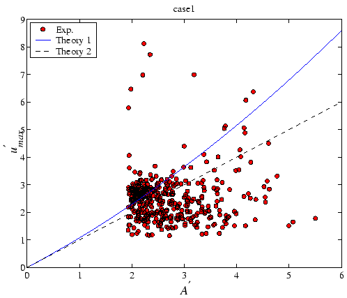
To check these assumptions and truncation,
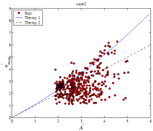
Fig.13 compares the measured relationship between
normalized wave crest amplitudes ![]() and the maximum horizontal
velocity
and the maximum horizontal
velocity
![]() with approximated solutions by Eq.(24)
and Eq.(25).
The approximated solution by Eq.(24) seems to
follow close to the maximum edge of the measured data, particularly in
Case 2.
Another approximated solution by Eq.(25) is
smaller than Eq.(24) and passes in the middle of the measured data.
It means that the maximum horizontal velocity
with approximated solutions by Eq.(24)
and Eq.(25).
The approximated solution by Eq.(24) seems to
follow close to the maximum edge of the measured data, particularly in
Case 2.
Another approximated solution by Eq.(25) is
smaller than Eq.(24) and passes in the middle of the measured data.
It means that the maximum horizontal velocity
![]() of measured data was
smaller than predicted by the linear sinusoidal wave theory.
Generally, the linear wave theory overestimates nonlinear random wave
kinematics.
Therefore these results are acceptable for us.
On the other hand, the scatter of
of measured data was
smaller than predicted by the linear sinusoidal wave theory.
Generally, the linear wave theory overestimates nonlinear random wave
kinematics.
Therefore these results are acceptable for us.
On the other hand, the scatter of
![]() in the figure for lower deck case
(Case 1) is larger than higher deck level case (Case 2).
Specially, some small amplitude waves have very high speed horizontal velocity
in Case 1.
These are collapsing waves that break on the deck and shoot across the
deck with very high speed.
The rest of the waves can be regarded as truncated wave that is clippedj
by the deck.
Therefore, we have to take into the consideration both of them, but
the collapsing waves are neglected in this paper.
in the figure for lower deck case
(Case 1) is larger than higher deck level case (Case 2).
Specially, some small amplitude waves have very high speed horizontal velocity
in Case 1.
These are collapsing waves that break on the deck and shoot across the
deck with very high speed.
The rest of the waves can be regarded as truncated wave that is clippedj
by the deck.
Therefore, we have to take into the consideration both of them, but
the collapsing waves are neglected in this paper.
Following this result, the assumptions of local sinusoidal wave theory for horizontal velocity component predicts the maximum value of horizontal velocity component on the deck, although, the assumptions cannot expect quantitatively agreement with the experimental data.
Solving Eq.(24) for ![]() , we have
, we have
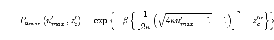 and is characteristic wave steepness.
Thus, the maximum horizontal velocity at wave crest:
and is characteristic wave steepness.
Thus, the maximum horizontal velocity at wave crest:
=11cm
![\epsfbox[50 185 547 592]{figures/theory2_Pu_z100.eps}](img155.png)
![\includegraphics[width=11cm]{figures/theory2_Pu_z100.eps}](img156.png) |
| =11cm
|
|
=11cm
![\epsfbox[50 185 547 592]{figures/expQpdfcase1.eps}](img114.png)
(a) Case 1.
=11cm ![\epsfbox[50 185 547 592]{figures/expQpdfcase2.eps}](img115.png)
(b) Case 2. |
|
=11cm
![\epsfbox[50 185 547 592]{figures/expQexccase1.eps}](img118.png)
(a) Case 1.
=11cm ![\epsfbox[50 185 547 592]{figures/expQexccase2.eps}](img119.png)
(b) Case 2. |
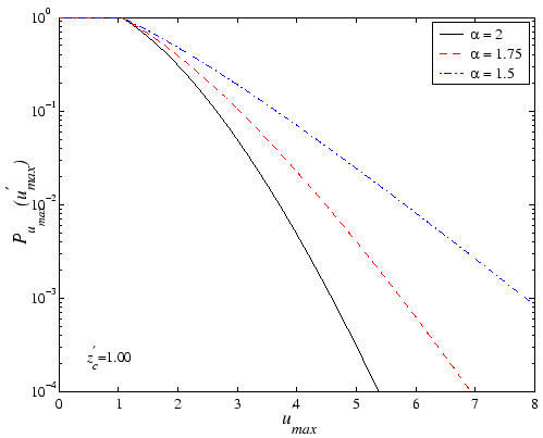
Fig.14 shows the sensitivity of the exceedance
probability of the modified Weibull
![]() distribution on
distribution on ![]() for the case of
for the case of ![]() =1.0 and
=1.0 and ![]() =0.1.
With a change in
=0.1.
With a change in ![]() from
from ![]() =1.5 to
=1.5 to ![]() =2,
the exceedance probability of
=2,
the exceedance probability of
![]() decreases one order of magnitude
at
decreases one order of magnitude
at
![]() and two orders of magnitude at
and two orders of magnitude at
 .
The
.
The
![]() decrease is slightly faster than overtopping volume
decrease is slightly faster than overtopping volume ![]() .
This is the reason why the function in the exponential in
Eq.(28) is proportional to
.
This is the reason why the function in the exponential in
Eq.(28) is proportional to
![]() .
The small characteristic wave steepness
.
The small characteristic wave steepness ![]() decrease exceedance
probability rapidly.
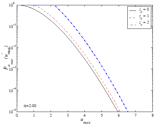
Fig.15 shows
the sensitivity of the exceedance probability of
decrease exceedance
probability rapidly.
Fig.15 shows
the sensitivity of the exceedance probability of
![]() to
the deck level
to
the deck level ![]() for the case of
for the case of ![]() =2.0.
With a change of
=2.0.
With a change of ![]() from
from ![]() =0 to
=0 to ![]() =2, the
exceedance probability decreases one order of
magnitude at
=2, the
exceedance probability decreases one order of
magnitude at
![]() and two orders of magnitude
at
and two orders of magnitude
at
 .
.
Fig.16 compares the PDF of the
normalized
![]() for the experimental results with the
modified Rayleigh
for the experimental results with the
modified Rayleigh
![]() distribution, Eq.(29),
and the modified Weibull
distribution, Eq.(29),
and the modified Weibull
![]() distribution, Eq.(27).
The both of theories for
distribution, Eq.(27).
The both of theories for
![]() show qualitatively worse
agreement with the experimental data.
One of reason of the differences between the theory and the measured
data is that the measured data include small
show qualitatively worse
agreement with the experimental data.
One of reason of the differences between the theory and the measured
data is that the measured data include small
![]() value that cannot expect
in the theory as shown in Fig.13.
Fig.17 compares the exceedance probability of
value that cannot expect
in the theory as shown in Fig.13.
Fig.17 compares the exceedance probability of
![]() for the experimental results with the modified Rayleigh
for the experimental results with the modified Rayleigh
![]() distribution, Eq.(30), and the modified Weibull
distribution, Eq.(30), and the modified Weibull
![]() distribution, Eq.(28).
The exceedance probability of measured
distribution, Eq.(28).
The exceedance probability of measured
![]() have two inflection
points for Case 1 and the both of the modified Weibull and Rayleigh
have two inflection
points for Case 1 and the both of the modified Weibull and Rayleigh
![]() distribution cannot predict this tendency.
The main reason of this strange
distribution cannot predict this tendency.
The main reason of this strange
![]() distribution is some small
amplitude waves have very high horizontal velocity in Case 1 as
explained before.
These are collapsing waves effects that break on the deck and shoot across the
deck with very high speed.
The number of collapsing waves on the deck is decreased as increasing
deck height.
Therefore, the modified Weibull
distribution is some small
amplitude waves have very high horizontal velocity in Case 1 as
explained before.
These are collapsing waves effects that break on the deck and shoot across the
deck with very high speed.
The number of collapsing waves on the deck is decreased as increasing
deck height.
Therefore, the modified Weibull
![]() distribution shows relatively
good agreement with the experimental data for high deck Case 2 in
comparison with Case 1,
although there is significant difference in the low velocity region.
Thus, the qualitative trends of high
distribution shows relatively
good agreement with the experimental data for high deck Case 2 in
comparison with Case 1,
although there is significant difference in the low velocity region.
Thus, the qualitative trends of high
![]() can be estimated by
Eq.(27) and (28) for middle deck
level case.
can be estimated by
Eq.(27) and (28) for middle deck
level case.
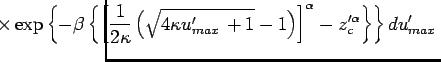
![$\displaystyle \frac{\alpha\beta}{\sqrt{4\kappa \ensuremath{u_{max}^\prime}\,+ 1...
... \sqrt{4\kappa \ensuremath{u_{max}^\prime}\,+ 1}- 1 )
\right]^{\alpha-1}
\!\!\!$](img148.png)
![$\displaystyle \hspace{-2.5cm}
\times
\exp\left\{
-\beta
\left\{
\left[
\frac{1}...
...ight]^{\alpha}
- z_c'^{\alpha}
\right\}
\right\}
d\ensuremath{u_{max}^\prime}\,$](img149.png)
![\begin{displaymath}
P_{\ensuremath{u_{max}}\,}(\ensuremath{u_{max}^\prime}\,,z_...
...\right)
\right]^{\alpha}
- z_c'^{\alpha}
\right\}
\right\}
\end{displaymath}](img150.png)
![$\displaystyle \hspace{-2.5cm}\times
\exp\left\{
-\frac{1}{8\kappa^2}
\left[
\le...
...1
\right)^2
- 4 \kappa^2 z_c'^2
\right]
\right\}
d\ensuremath{u_{max}^\prime}\,$](img153.png)
![\begin{displaymath}
P^R_{\ensuremath{u_{max}}\,}(\ensuremath{u_{max}^\prime}\,,...
...e}\,+ 1}- 1
\right)^2
- 4 \kappa^2 z_c'^2
\right]
\right\}
\end{displaymath}](img154.png)