The overtopping volume, ![]() , can be defined as the volume of water
column above the deck level, shown schematically
in Fig.3.
The overtopping volume
, can be defined as the volume of water
column above the deck level, shown schematically
in Fig.3.
The overtopping volume ![]() only depends on spatial surface profile, if
the deck is thin compared to the incident wave amplitude.
Therefore, if the spatial wave profile is known, it is possible to
calculate the overtopping volume
only depends on spatial surface profile, if
the deck is thin compared to the incident wave amplitude.
Therefore, if the spatial wave profile is known, it is possible to
calculate the overtopping volume ![]() accurately.
However, there is some difficulty to estimate the spatial profile of
random waves.
Thus, following Mori and Cox (2003), the overtopping volume
accurately.
However, there is some difficulty to estimate the spatial profile of
random waves.
Thus, following Mori and Cox (2003), the overtopping volume ![]() is calculated by the following assumptions and procedure.
First, the profile of the individual wave crest is assumed to be a sinusoidal wave locally.
Then, if the deck level
is calculated by the following assumptions and procedure.
First, the profile of the individual wave crest is assumed to be a sinusoidal wave locally.
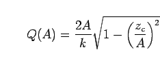
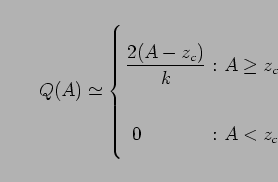
Then, if the deck level ![]() is given and the crest amplitude
is given and the crest amplitude ![]() is
known, the volume of water column above deck level,
is
known, the volume of water column above deck level, ![]() , is simply calculated by
, is simply calculated by
|
=11cm
![\includegraphics[width=11cm]{figures/theory_amplitude-volume.eps}](img89.png)
|
|
=11cm
![\includegraphics[width=11cm]{figures/H-T.eps}](img91.png)
|
|
=11cm
![\epsfbox[47 184 550 606]{figures/exp_amp-Q2_case1.eps}](img92.png)
(a) Case 1.
=11cm ![\epsfbox[47 184 550 606]{figures/exp_amp-Q2_case2.eps}](img93.png)
(b) Case 2. |
Before formulate the PDF of overtopping volume model, it is
necessary to check some of the basic assumptions used though
Eq.(12) to Eq.(14).
The local wave number ![]() was regarded as a constant above formulation.
Empirically, the assumptions of a locally sinusoidal wave
crest profile and local wave number are applicable for
narrow banded spectra.
Evidently from Eq.(13), the wavelength or period
is important in estimating the overtopping for extreme waves.
Generally, the relationship between wave period and wave height for
random waves has a linear trend for small value of wave height, and the
wave period becomes relatively constant for large amplitude waves.
Therefore, the constant local wave number assumption is more
crude for small amplitude waves but it is reasonably acceptable
for large amplitude waves (e.g. Goda, 1985).
Fig.7 shows experimental results of the
relationship between
was regarded as a constant above formulation.
Empirically, the assumptions of a locally sinusoidal wave
crest profile and local wave number are applicable for
narrow banded spectra.
Evidently from Eq.(13), the wavelength or period
is important in estimating the overtopping for extreme waves.
Generally, the relationship between wave period and wave height for
random waves has a linear trend for small value of wave height, and the
wave period becomes relatively constant for large amplitude waves.
Therefore, the constant local wave number assumption is more
crude for small amplitude waves but it is reasonably acceptable
for large amplitude waves (e.g. Goda, 1985).
Fig.7 shows experimental results of the
relationship between ![]() and
and ![]() .
For large wave height (
.
For large wave height (
![]() roughly),
roughly), ![]() can be regarded as approximately
constant,
can be regarded as approximately
constant,
 .
Thus, the theory of overtopping is more accurate for
larger amplitude waves and it is less valid for
small amplitude waves.
In this study, local wave number is assumed constant
and
.
Thus, the theory of overtopping is more accurate for
larger amplitude waves and it is less valid for
small amplitude waves.
In this study, local wave number is assumed constant
and ![]() is regarded as
is regarded as
 calculated
by the linear dispersion relationship with
calculated
by the linear dispersion relationship with ![]() .
Of course, the assumption of
is not a necessary
condition for the assumption of sinusoidal wave profile.
.
Of course, the assumption of
is not a necessary
condition for the assumption of sinusoidal wave profile.
To check the local sinusoidal wave profile assumption,
Fig.8 compares the measured relationship between
normalized wave crest amplitudes ![]() and overtopping volume
and overtopping volume ![]() with exact solution, Eq.(12), and approximated solution,
Eq.(13).
The approximated solution, Eq.(13), gives better
agreement with the measured data than the exact solution,
Eq.(13).
It means that the spatial profile of mechanically generated waves
in the flume was slimmer than sinusoidal wave.
Eq.(13) shows better agreement with high deck level
case (Case 2) than low deck level case (Case 1).
The correlation coefficients between Eq.(13) and
the experimental results are 0.75 for Case 1 and 0.85 for Case 2.
As a result, the assumptions of the local sinusoidal wave profile and
constant wave number are acceptable for large amplitude waves, especially relatively high deck level condition.
with exact solution, Eq.(12), and approximated solution,
Eq.(13).
The approximated solution, Eq.(13), gives better
agreement with the measured data than the exact solution,
Eq.(13).
It means that the spatial profile of mechanically generated waves
in the flume was slimmer than sinusoidal wave.
Eq.(13) shows better agreement with high deck level
case (Case 2) than low deck level case (Case 1).
The correlation coefficients between Eq.(13) and
the experimental results are 0.75 for Case 1 and 0.85 for Case 2.
As a result, the assumptions of the local sinusoidal wave profile and
constant wave number are acceptable for large amplitude waves, especially relatively high deck level condition.
From Eq.(14), the inverse relationship between ![]() and
and ![]() is given by
is given by
 .
Therefore, number of overtopping events is different from number of
incident wave events.
.
Therefore, number of overtopping events is different from number of
incident wave events.
Thus, the PDF of the modified Weibull overtopping distribution has a similar profile compared to the Rayleigh distribution for wave amplitude.
This implies that wave nonlinearities (or spectrum band width) directly
affects the overtopping volume via ![]() in Eq.(16) to (17).
in Eq.(16) to (17).
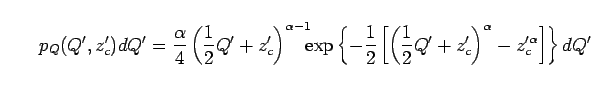
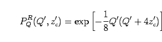
For the special case of ![]() =2 and
=2 and ![]() =1/2 which is the Rayleigh
condition for the wave amplitude distribution, Eq.(16)
and (17) are simplified as
=1/2 which is the Rayleigh
condition for the wave amplitude distribution, Eq.(16)
and (17) are simplified as
| =11cm
|
Fig.9 shows
the sensitivity of the exceedance probability
of the modified Weibull overtopping distribution
on ![]() for the case of
for the case of ![]() =1.0.
With a change in
=1.0.
With a change in ![]() from
from ![]() =1.5 to
=1.5 to ![]() =2,
the exceedance probability of
=2,
the exceedance probability of ![]() decreases one order of magnitude
at
decreases one order of magnitude
at ![]() and two orders of magnitude
at
and two orders of magnitude
at ![]() .
Fig.10 shows
the sensitivity of the exceedance probability of
.
Fig.10 shows
the sensitivity of the exceedance probability of ![]() to
the deck level
to
the deck level ![]() for the case of
for the case of ![]() =2.0. With a change of
=2.0. With a change of
![]() from
from ![]() =0 to
=0 to ![]() =2, the
exceedance probability decreases one order of
magnitude at
=2, the
exceedance probability decreases one order of
magnitude at ![]() and two orders of magnitude
at
and two orders of magnitude
at ![]() .
.
|
=11cm
![\epsfbox[50 185 547 592]{figures/expQpdfcase1.eps}](img114.png)
(a) Case 1.
=11cm ![\epsfbox[50 185 547 592]{figures/expQpdfcase2.eps}](img115.png)
(b) Case 2. |
|
=11cm
![\epsfbox[50 185 547 592]{figures/expQexccase1.eps}](img118.png)
(a) Case 1.
=11cm ![\epsfbox[50 185 547 592]{figures/expQexccase2.eps}](img119.png)
(b) Case 2. |
Fig.11 compares the PDF of the
normalized wave overtopping for the experimental results with the
modified Rayleigh overtopping
distribution Eq.(18), and the modified Weibull overtopping distribution Eq.(16).
The modified Weibull overtopping distribution shows
qualitatively better agreement
with the experimental data than the modified Rayleigh overtopping distribution, particularly for larger values of ![]() .
Fig.12 compares the exceedance probability of wave
overtopping for the experimental results with the modified Rayleigh
overtopping distribution Eq.(19) and the modified Weibull
overtopping distribution
Eq.(17).
The modified Rayleigh overtopping distribution shows fair agreement
with the experimental data for small values of
.
Fig.12 compares the exceedance probability of wave
overtopping for the experimental results with the modified Rayleigh
overtopping distribution Eq.(19) and the modified Weibull
overtopping distribution
Eq.(17).
The modified Rayleigh overtopping distribution shows fair agreement
with the experimental data for small values of ![]() , and the modified
Weibull overtopping distribution shows particularly good agreement
with the experimental data for larger values of
, and the modified
Weibull overtopping distribution shows particularly good agreement
with the experimental data for larger values of ![]() .
This is reasonable result because the main purpose to use the Weibull
distribution is to estimate accurately large wave events.
However, the number of overtopping event is insufficient to compare quantitatively,
but the qualitative trends of the overtopping volume can be estimated by
Eq.(16) and (17).
.
This is reasonable result because the main purpose to use the Weibull
distribution is to estimate accurately large wave events.
However, the number of overtopping event is insufficient to compare quantitatively,
but the qualitative trends of the overtopping volume can be estimated by
Eq.(16) and (17).
![\begin{displaymath}
p_Q(Q',z_c')dQ'
=
\frac{\alpha}{4}
\left(
\frac{1}{2}Q'...
...Q' + z_c'\right)^{\alpha}
- z_c'^\alpha
\right]
\right\}dQ'
\end{displaymath}](img100.png)
![\begin{displaymath}
P_Q(Q',z_c')
=
\exp\left\{
-\frac{1}{2}
\left[
\left(\...
...{2}Q' + z_c'\right)^{\alpha}
- z_c'^\alpha
\right]
\right\}
\end{displaymath}](img102.png)
![\begin{displaymath}
P_Q^R(Q',z_c')
=
\exp\left[
- \frac{1}{8}
Q'(Q' + 4z_c')
\right]
\end{displaymath}](img105.png)
![\includegraphics[width=11cm]{figures/theory2_PQ_z100.eps}](img107.png)